2013
In Proceedings of GALA,
2013
International Journal of Computer Assisted Radiology and Surgery,
2013
Int J Biomed Imaging,
2013
In Proceedings of ICT Open,
2013
2012
IEEE Transactions on Visualization and Computer Graphics,
2012
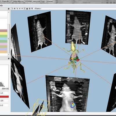
In Proceedings of TOPIM - Hot Topics in Molecular Imaging,
2012
In Proceedings of IVA,
2012
Lecture Notes in Geoinformation and Cartography,
2012
In Proceedings of Vision, Modeling, and Visualization,
2012
Comput Animat Virtual Worlds,
2012
SIAM J Imaging Sci,
2012
IEEE Transactions on Visualization and Computer Graphics,
2012
![Real-time rendering applications exhibit a considerable amount of spatio-temporal coherence. This is true for camera motion, as in the Parthenon sequence (left), as well as animated scenes such as the Heroine (middle) and Ninja (right) sequences. Diagrams to the right of each rendering show disoccluded points in red, in contrast to points that were visible in the previous frame, which are shown in green (i.e. green points are available for reuse). [Images courtesy of Advanced Micro Devices, Inc., Sunnyvale, California, USA]](https://publications.graphics.tudelft.nl/rails/active_storage/representations/redirect/eyJfcmFpbHMiOnsibWVzc2FnZSI6IkJBaHBBdVFJIiwiZXhwIjpudWxsLCJwdXIiOiJibG9iX2lkIn19--7e1125f607030dc5d6de0c68836a681f5432efb9/eyJfcmFpbHMiOnsibWVzc2FnZSI6IkJBaDdCem9MWm05eWJXRjBTU0lJY0c1bkJqb0dSVlE2RTNKbGMybDZaVjkwYjE5bWFXeHNXd2RwQXBBQmFRS1FBUT09IiwiZXhwIjpudWxsLCJwdXIiOiJ2YXJpYXRpb24ifX0=--8786188a9503cffd21c59bbcd5519930c73c621f/greenmotion-teaser.png)